sktime is 1.0

sktime is 1.0, and the number now carries a commitment: it tells you what an upgrade is allowed to do to your code. sktime follows semantic versioning, so a patch release carries backward compatible bug fixes and nothing else, a minor release adds functionality, and an incompatible API change waits for a minor or major release.

The deprecation cycle in front of such a change is not new. sktime has warned before it removed or renamed anything for years, a full minor cycle ahead, so you hear about a change from a warning in your own test run rather than from a red build. What 1.0 adds is that the version number itself now tells you which changes are even permitted, which makes every interface in this post one you can pin a production system to.

That promise is worth what the maintenance behind it is worth. sktime is developed by a core team under a public governance model, on a regular release schedule, and the same people take on enterprise work on request: running sktime in production inside a company, support with an SLA, forward-deployed engineers, training, and consulting.

Here is what recently shipped:

That window is why this post covers three releases rather than one: 1.0.0 set the new API and opened it, 1.0.2 expanded on it, and 1.1.0 closed it. Everything below is in 1.1.0, and where a feature arrived after 1.0.0, the text says which release brought it.

Foundation models: one interface, >30 families, >100 models

A pretrained foundation model, on your own data, in four lines:

from sktime.datasets import load_airline
from sktime.forecasting.chronos2 import Chronos2Forecaster

y = load_airline()

forecaster = Chronos2Forecaster("amazon/chronos-2")
forecaster.fit(y, fh=range(1, 13))
y_pred = forecaster.predict()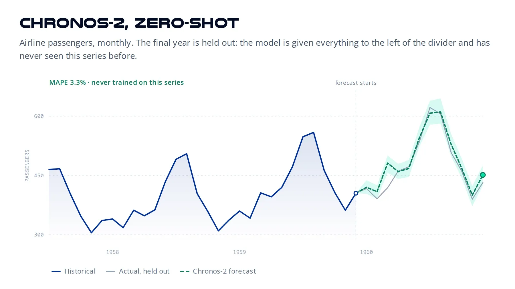

You can see how little it takes to put a foundation model on your own series. And because the sktime devs did the plumbing, every other one of them follows the exact same logic: import a different class, and that is it. Swap Amazon’s Chronos-2 for Google’s TimesFM 2.5 and nothing else in your code moves, even though the two come from different vendors, sit on different backing libraries, and expect their inputs in different shapes:

from sktime.datasets import load_airline
from sktime.forecasting.chronos2 import Chronos2Forecaster
from sktime.forecasting.timesfm2 import TimesFM2Forecaster

y = load_airline()
fh = range(1, 13)

for forecaster in [
    Chronos2Forecaster("amazon/chronos-2"),
    TimesFM2Forecaster("google/timesfm-2.5-200m-transformers"),
]:
    forecaster.fit(y, fh=fh)
    print(forecaster.predict().head(3))

In a world without sktime, you would do this by hand. Here is the vendor-native way to get three points out of IBM’s Tiny Time Mixer:

import pandas as pd
from tsfm_public.toolkit.get_model import get_model
from tsfm_public.toolkit.time_series_forecasting_pipeline import (
    TimeSeriesForecastingPipeline,
)
from tsfm_public.toolkit.time_series_preprocessor import TimeSeriesPreprocessor

y = pd.Series([1, 2, 3, 4, 5])
df = pd.DataFrame(
    {
        "timestamp": pd.date_range("2024-01-01", periods=len(y), freq="D"),
        "value": y.to_numpy(),
    }
)

model = get_model(
    "ibm-research/ttm-r3",
    context_length=52,
    prediction_length=3,
    model_revision="52-16-dec-52-lite-r3",
)
preprocessor = TimeSeriesPreprocessor(
    timestamp_column="timestamp",
    target_columns=["value"],
    context_length=52,
    prediction_length=3,
    scaling=False,
    freq="D",
)
preprocessor.train(df)
pipe = TimeSeriesForecastingPipeline(
    model=model,
    feature_extractor=preprocessor,
    prediction_length=3,
    explode_forecasts=True,
    add_known_ground_truth=False,
)
print(pipe(df))

And the same thing in sktime:

import pandas as pd
from sktime.forecasting.ttm import TinyTimeMixerForecaster

y = pd.Series([1, 2, 3, 4, 5])
forecaster = TinyTimeMixerForecaster(
    model_path="ibm-research/ttm-r3", revision="52-16-dec-52-lite-r3"
)
forecaster.fit(y, fh=[1, 2, 3])
print(forecaster.predict())
# 5    6.072927
# 6    7.396875
# 7    8.460439

Same model, same three numbers. The context length and the preprocessor did not go away; they moved behind the interface, where they are defaults you can override rather than boilerplate you have to write. However, the checkpoint revision is the one thing you still name yourself, because it selects the model: leave it off and you get the default main checkpoint, which is a different set of weights and a different answer.

Twenty-nine forecasters work that way today, and each one is an interface to a model family rather than to a single checkpoint, so the number of individual models you can reach through them is a good deal larger. The table below is ordered by how much the underlying checkpoint is actually used. The Added column says which release brought each one in; the eighteen marked in green are new with 1.0. Each name links to its API reference, where you will find the default checkpoint and the extra dependencies it needs:

Estimator	Added	Model year	Downloads / mo
Chronos2Forecaster	1.0.0	2025	23.8M
KronosForecaster	1.0.0	2025	1.2M
ChronosForecaster	earlier	2024	1.0M
TiRexForecaster	earlier	2025	423K
TinyTimeMixerForecaster	earlier	2024	329K
Moirai2Forecaster	1.0.2	2025	192K
Toto2Forecaster	1.0.2	2026	107K
TimeMoEForecaster	earlier	2024	106K
TotoForecaster	earlier	2025	83K
MantisForecaster	1.0.0	2025	80K
FlowStateForecaster	1.0.0	2025	72K
TimesFM2Forecaster	1.0.0	2026	63K
SundialForecaster	1.0.2	2025	41K
MomentFMForecaster	earlier	2024	36K
MOIRAIForecaster	earlier	2024	32K
AuroraForecaster	1.0.2	2026	6.3K
TimerForecaster	1.0.0	2024	4.6K
PatchTSMixerForecaster	1.0.0	2023	3.1K
TimerS1Forecaster	1.0.0	2026	1.1K
CiscoTSMForecaster	1.0.2	2026	903
FalconTSTForecaster	1.0.0	2025	743
PatchTSTForecaster	earlier	2023	606
TimesFMForecaster	earlier	2024	600
MIRAForecaster	1.0.2	2025	579
WindFMForecaster	1.0.2	2025	567
LagLlamaForecaster	1.0.0	2024	n/a
FalconXForecaster	1.0.2	2026	remote API

Two more are adapters rather than single models, so a download count would not mean much: HFTransformersForecaster wraps any compatible Hugging Face time-series checkpoint, and TimeLLMForecaster reprograms a general-purpose language model as a forecaster.

Forecasting is not the only task. 1.0 also brings MantisClassifier and TSPulseClassifier for classification, plus MomentFMAnomalyDetector and TSPulseAnomalyDetector for anomaly detection. Same fit and predict, different job. That makes 33 model families across three tasks, 22 of them new in the 1.0 series.

Browse every foundation model in the API reference→

Global forecasting, and pretraining on your own data

All of those models still leave one thing open: every one of them arrives pretrained on somebody else’s data, and zero-shot only gets you so far. So 1.0 also introduces a pretraining API, led by Simon Blanke (@SimonBlanke) with Benedikt Heidrich (@benHeid), Felipe Angelim (@felipeangelimvieira), and Franz Király (@fkiraly).

Forecasters carrying the capability:pretrain tag do exactly that: the fit after pretrain fine-tunes rather than resets, so the pretrained weights are kept. The panel is paid for once, and each series you forecast afterwards is a cheap fit and predict on top of it:

from sktime.datasets import load_hierarchical_sales_toydata
from sktime.forecasting.ltsf import LTSFLinearForecaster

y_panel = load_hierarchical_sales_toydata()

forecaster = LTSFLinearForecaster(seq_len=12, pred_len=6, num_epochs=5, batch_size=8)
forecaster.pretrain(y_panel)

y_target = y_panel.loc[y_panel.index.droplevel(-1).unique()[0]]
forecaster.fit(y_target, fh=range(1, 7))
y_pred = forecaster.predict()

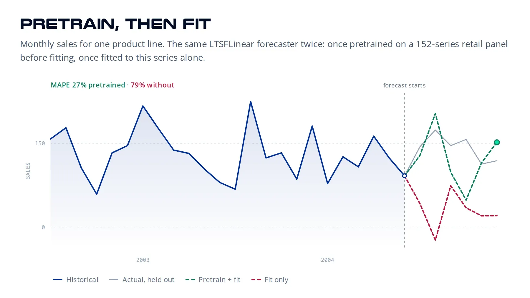
What that buys you shows up when the target series is short. Below is one product line’s monthly sales, six months held out, forecast twice by the same LTSFLinearForecaster: once pretrained on a panel of 152 unrelated Australian retail series before fitting, once fitted to the target series and nothing else. Five epochs each, so neither number is a benchmark result. The gap between them is the point, and the pretraining notebook runs the whole comparison:

What this replaces is the old global forecasting API. Before 1.0, that was two methods doing each other’s jobs. The panel went to fit, and the series you actually wanted forecast went to predict, as a y argument that temporarily re-pointed the fitted forecaster at data it had never seen. It worked, but y meant something different depending on which method you handed it to, and it needed a separate base class that pipelines and tuners had to know about. 1.1.0 splits the two roles: pretrain takes the panel, fit takes the series, and predict goes back to taking no data at all.

Two things here sound alike and are not. Fitting a forecaster on a panel and predicting every series in it works as it always did, and needs nothing from this section. The case that changed is the other one: learn from a panel, then forecast a series the fit never saw. That used to mean handing the new series to predict. Now the panel goes to pretrain and the new series goes to fit, which is the method that is meant to see data in the first place.

Fourteen forecasters carry the capability:pretrain tag in 1.1.0, among them the LTSF linear family, SCINetForecaster, TimesFM2Forecaster, and, from 1.0.2, SundialForecaster and TinyTimeMixerForecaster. To list them all:

from sktime.registry import all_estimators

all_estimators(filter_tags={"capability:pretrain": True})

Deep learning on torch

Deep learning in sktime used to mean Keras and TensorFlow. Since 1.0 you can do all of it on torch instead, the dependency the foundation models above already pull in. Nine classifiers and nine regressors gained native torch implementations, each marked with a Torch suffix. The TensorFlow versions stay where they are, so nothing you already run breaks. From sktime.classification.deep_learning: CNNClassifierTorch, InceptionTimeClassifierTorch, MACNNClassifierTorch, MCDCNNClassifierTorch, SimpleRNNClassifierTorch, and TapNetClassifierTorch. ConvTran, LSTM-FCN, and MLP variants live in their own submodules, and sktime.regression.deep_learning exports the mirror-image set, plus MLPRegressorTorch.

from sktime.classification.deep_learning import CNNClassifierTorch
from sktime.datasets import load_unit_test

X_train, y_train = load_unit_test(split="train")
X_test, y_test = load_unit_test(split="test")

clf = CNNClassifierTorch(num_epochs=20, batch_size=8)
clf.fit(X_train, y_train)
y_pred = clf.predict(X_test)

You pass loss functions, optimizers, and callbacks as strings or callables. Most of the set, though not CNNClassifierTorch, also takes a metrics argument that accepts torchmetrics metrics directly.

Enhanced benchmarking

Foundation models, a pretraining API, and an agent that generates pipelines all raise the same question: which of them is actually better on your data? That is what the benchmarking rewrite is for. It is the largest single overhaul in this release, from Jigyasu (@jgyasu), with the post-hoc analysis tools from Yash Sangwan (@yash-sangwan).

A benchmark is a set of estimators, a task, and a metric. Seasonal naive against a small foundation model on the airline data, five expanding windows:

from sktime.benchmarking.forecasting import ForecastingBenchmark
from sktime.datasets import Airline
from sktime.forecasting.chronos import ChronosForecaster
from sktime.forecasting.naive import NaiveForecaster
from sktime.performance_metrics.forecasting import MeanAbsolutePercentageError
from sktime.split import ExpandingWindowSplitter

benchmark = ForecastingBenchmark()

benchmark.add(NaiveForecaster(strategy="last", sp=12))
benchmark.add(ChronosForecaster("amazon/chronos-bolt-tiny"))
benchmark.add(
    (
        Airline(),
        MeanAbsolutePercentageError(),
        ExpandingWindowSplitter(initial_window=24, step_length=24, fh=12),
    )
)

results = benchmark.run()

results is a DataFrame with one row per estimator. Each metric contributes a column per fold plus a mean and a standard deviation, and fit and predict times come along the same way. What you actually read is smaller, so rank by the mean:

metric = "MeanAbsolutePercentageError"
results.set_index("model_id")[f"{metric}_mean"].sort_values()
# model_id
# NaiveForecaster      0.135761
# ChronosForecaster    0.157366
# Name: MeanAbsolutePercentageError_mean, dtype: float64

Estimator	MAPE (mean ± std)	Fit time (s)
NaiveForecaster	0.1358 ± 0.0323	0.004
ChronosForecaster	0.1574 ± 0.0929	0.482

Those add calls are the first change. Since 1.0.0, add takes whatever you give it and works out what it is: an estimator, a list or dict of estimators, a dataset object, a metric, a cross-validation splitter, or a (dataset, metric, splitter) triple in any order. On top of that sits a new object type, the catalogue, a declarative and inspectable collection of estimators, datasets, metrics, and splitters that you hand to a benchmark whole. Seven ship with 1.0: the six M4 competition catalogues and BakeOffCatalogue, which covers the 2017 time series classification bake-off with 85 datasets and 13 classifiers.

A catalogue is worth opening before you run it. The M4 yearly one holds the competition’s nine statistical baselines, with the exact parameters each was run with:

from sktime.catalogues import M4CompetitionCatalogueYearly

M4CompetitionCatalogueYearly().get("forecaster")
# [{'Naive_1': "NaiveForecaster(strategy='last')"},
#  {'SES': 'ExponentialSmoothing(trend=None, seasonal=None)'},
#  {'Holt': "ExponentialSmoothing(trend='add', seasonal=None)"},
#  {'Damped': "ExponentialSmoothing(trend='add', damped_trend=True)"},
#  {'Theta': 'ThetaForecaster()'},
#  {'AutoARIMA': 'AutoARIMA()'},
#  {'AutoETS': 'AutoETS()'},
#  {'Comb': 'EnsembleForecaster(...)'},  # abbreviated: mean of SES, Holt, Damped
#  {'Naive_S': "NaiveForecaster(strategy='last', sp=1)"}]

The dataset and the competition’s three metrics sit in the same object, under get("dataset") and get("metric"). So you can see what you will be compared against, and what you will be scored on, before spending the compute.

Reproducing those baselines is then a catalogue, a splitter, and a path:

from sktime.benchmarking.forecasting import ForecastingBenchmark
from sktime.catalogues import M4CompetitionCatalogueYearly
from sktime.split import ExpandingWindowSplitter

catalogue = M4CompetitionCatalogueYearly()
benchmark = ForecastingBenchmark(backend="loky")

benchmark.add(catalogue)
benchmark.add(ExpandingWindowSplitter(initial_window=12, step_length=2, fh=6))

results = benchmark.run("./m4_yearly_results.csv")

Add your own estimator to that same benchmark with one more add, and you have a like-for-like comparison against published baselines. The M4 competition notebook walks through the whole run.

The second change, also 1.0.2, matters once a run takes hours. A benchmark is fault tolerant: if one task-estimator pair raises, that pair is recorded and the run carries on, with a warning summarising the failures at the end and the details in benchmark.failed_experiments. It is also crash safe. Each completed pair is written out as it finishes, into a .parts/ directory beside your output file, so pointing run at the same path after a crash, a timeout, or a power cut picks up where it stopped instead of starting over. Rerunning something deliberately is force_rerun="all", or a list of estimator IDs to redo. For cluster runs, sktime-benchmark is a worked Slurm example.

The analysis tools, new in 1.0.2, read that results frame directly, either the frame itself or the path it was written to. They compare estimators across datasets, so they want a run with several tasks in it. Here results holds four classical forecasters over Airline, Lynx, and ShampooSales:

from sktime.benchmarking.analysis import AverageRank, FriedmanTest

metric = "MeanAbsolutePercentageError"

AverageRank(metric=metric).evaluate(results)
#   model_id      rank
# 0    Trend  1.000000
# 1    Theta  2.666667
# 2    Naive  3.000000
# 3     Mean  3.333333

FriedmanTest(metric=metric).evaluate(results)
#    statistic   p_value
# 0        5.8  0.121757

TrendForecaster ranks first, and the Friedman test declines to call that a real difference, which is the right answer on three datasets. A post-hoc NemenyiTest would only be worth running once the omnibus test rejects.

AverageRank, FriedmanTest, NemenyiTest, WilcoxonSignedRankTest, SignTest, RankSumTest, TwoSampleTTest, and CriticalDifferenceDiagram are all available from sktime.benchmarking.analysis. One caveat: the analyzers need a complete score matrix, so finish or filter a run with failed experiments before you rank it.

Agentic forecasting

Picking the right model out of the foundation-model line-up above, then the right pipeline around it, is work. 1.0 will do that part for you as well.

AutoResearchForecaster, contributed by Benedikt Heidrich (@benHeid), hands pipeline design to a language model. It proposes candidate pipelines as specifications, builds them through sktime’s registry, evaluates each one against your data with a real cross-validation splitter, then uses those scores to propose better ones. After fit, the pipeline it settled on is a normal sktime forecaster sitting in best_forecaster_:

from sktime.datasets import load_airline
from sktime.forecasting.agentic import AutoResearchForecaster
from sktime.split import SingleWindowSplitter

y = load_airline()

forecaster = AutoResearchForecaster(
    cv=SingleWindowSplitter(fh=[1, 2, 3]),
    model="openai/gpt-4o-mini",
    n_iterations=2,
    n_blueprints=3,
)
forecaster.fit(y, fh=[1, 2, 3])
y_pred = forecaster.predict(fh=[1, 2, 3])

forecaster.best_forecaster_
forecaster.blueprint_history_

How AutoResearchForecaster builds a pipeline

1Training data

• The target series y, plus optional exogenous X
• A dataset description: plain statistics, a vision model's read of a plot, or the plot image itself, depending on description_method

2Prompt context

• System prompt: the blueprint format, the spec rules, and every available sktime forecaster and transformer class name
• User message: the dataset description, and the chart image if the model can see one

Repeated n_iterations times

GenerateLLM call

The LLM proposes n_blueprints pipeline blueprints, each with a name, a reason, and a spec handed to craft().

Detrender() * AutoARIMA()

Evaluatesktime

craft() builds each spec into a real forecaster, evaluate() scores it on a cross-validation split. A failure does not stop the run: the LLM gets n_fix_attempts tries to repair a broken spec.

score = MAPE = 0.0421

RefineLLM call

The LLM sees every blueprint tried so far, ranked by score, and is asked to improve the best one, fix the failures, and try new combinations.

best_score_ = 0.0421
rank all blueprints tried

The ranked history feeds the next round of Generate

3Select and refit

• best_blueprint_: the best spec across every iteration
• Rebuilt with craft() and refit on the full training set, which gives you best_forecaster_

4Forecast

• predict(fh) returns the forecast from best_forecaster_
• summary() returns every blueprint tried, ranked by score

Model calls go through litellm, so any provider it supports works. Set the matching API key in your environment. Two things to plan for: the search spends tokens, and with a language model in the loop, two runs need not settle on the same pipeline. However, the search space is sktime’s own registry, so whatever the agent hands back is an ordinary sktime object, inspectable, serialisable, and runnable afterwards without a single model call.

Alongside this, sktime-mcp exposes sktime’s registry and semantics to any MCP-capable assistant, so an LLM can discover and reason about estimators directly. It is a separate package with its own release cycle, contributed by Shashank Shekhar Singh.

Further changes

The four things above are what we would put on the poster, but a major release moves more than four things. The rest of 1.0 is a solid round of classical estimators and metrics, and the interface fixes that a major version is the right place to make.

Statistical and classical additions in 1.0.2

The Arps decline curve forecasters, ArpsExponential, ArpsHyperbolic, and ArpsHarmonic in sktime.forecasting.arps_dca, come from Santiago Cuervo (@scuervo91). They bring the standard petroleum production decline models into sktime, with probabilistic forecasts via an empirical distribution:

import numpy as np
import pandas as pd
from sktime.forecasting.arps_dca import ArpsHyperbolic

# three years of monthly production from a declining well
t = np.arange(36)
y = pd.Series(
    1000 / (1 + 0.8 * 0.12 * t) ** (1 / 0.8),
    index=pd.period_range("2023-01", periods=36, freq="M"),
)

forecaster = ArpsHyperbolic()
forecaster.fit(y, fh=range(1, 13))
y_pred = forecaster.predict()
y_pred_int = forecaster.predict_interval(coverage=0.9)

Also new: HyperTreeNetARForecaster, interfacing hypertrees-forecasting; seven accuracy metrics from Chen and Yang (2004) in sktime.performance_metrics.forecasting, from Michael Ellis (@michaelellis003), including RMSEnormalizedByIQR, TheilU2, and three KL-divergence variants; MiniRocketMultivariateCython, a numba-free MiniRocket with no JIT warmup and threaded n_jobs; and EvoForestTSWM, a closed-form feature extractor.

From 1.0.0, on the statistical side: Johansen cointegration and impulse-response functions for VAR-family models in sktime.param_est, from @OldPatrick, and tsfeatures, tsfel, and DegreeDayFeatures feature extractors from Faakhir Zahid (@Faakhir30) and Zack Stinnett (@zstinnett3). 1.0.0 also merged skchange into sktime, so its change-point and anomaly detection algorithms are now native sktime.detection estimators.

What changed, and what to do about it

Five of those fixes are worth knowing about before you upgrade.

Integer forecasting horizons are unambiguous. fh=3 now means [1, 2, 3], forecast the next three periods. It previously meant the third period only. If you pass a bare integer anywhere, check it:

from sktime.datasets import load_airline
from sktime.forecasting.naive import NaiveForecaster

y = load_airline()  # monthly, ends 1960-12
NaiveForecaster().fit(y, fh=3).predict()
# 1961-01    432.0
# 1961-02    432.0
# 1961-03    432.0
#
# before 1.0, the same call returned one row: 1961-03

Capability tags are consistent. ignores-exogeneous-X became capability:exogenous, and univariate-only became capability:multivariate. Both flip the boolean, because the new names say what an estimator can do rather than what it cannot. scitype:y is replaced by capability:multivariate too. This matters if you query tags or maintain third-party estimators.

The module layout is flatter. sktime.transformations.series.* and sktime.transformations.panel.* are gone; import from sktime.transformations.* directly. sktime.detection is flattened the same way, and the old series-annotator type is now detector. The old import paths keep working through the 1.x series.

Installs are leaner. all_extras no longer drags in every estimator-specific dependency. Those are declared per estimator in the python_dependencies tag and installed when you need them, which is what makes a foundation model line-up that size practical. Two knock-on removals: the vendored sktime.libs.pykalman (install pykalman yourself) and the deprecated ColumnTransformer.

If you extend sktime, one more: __init__ is now reserved for assigning arguments to self. Dynamic tags go in __dynamic_tags__ and other setup in __post_init__.

The capability:global_forecasting tag is deprecated too. With the legacy global forecasting API gone, reading the old tag warns until it is removed in 1.2.0, and tag queries are not redirected, because estimators from earlier versions carry both tags at once. So filter on capability:pretrain.

Those deprecations, and the tag aliases above, are the whole of 1.1.0, released two days after 1.0.2. Which is why upgrading through 1.0.2 first pays off: if it runs without deprecation warnings, 1.1.0 is a no-op for you.

Full detail is in the changelog.

Get started

pip install --upgrade sktime

• New to sktime? Start with the tutorials and example notebooks.
• Writing your own estimator? See the extension templates.
• Looking something up? The API reference covers every one of them.

Built in the open

sktime is BSD-licensed, openly governed, and interoperable across the PyData ecosystem. As of 1.1.0 it carries 616 estimators, among them 153 forecasters, 150 transformers, 77 classifiers, 46 metrics, 30 regressors, and 28 detectors, and it is downloaded about a million times a month from PyPI. 636 people have contributed commits.

Code is not the only contribution that counts. sktime follows the all-contributors specification and recognises documentation, tutorials, reviews, issue triage, event organising, and design. We run a mentoring programme and weekly community sessions, and there is always a stack of good first issues.

• Contributing guide
• Discord

Thank you

113 people contributed to 1.0.0, 1.0.2, and 1.1.0, several for the first time:

@12jaspreetsingh, @Abelarm, @abhimanyudalal1, @adan-shahid, @adrynalean, @algojogacor, @alphaleporus, @AMBRA7592, @aminehd, @Aniketsy, @Ankit-1204, @archittmittal, @Ask-812, @AYUSH27112021, @AyushI7G, @benHeid, @Chetansahney, @CloseChoice, @crocmons, @DCchoudhury15, @Deep-Axe, @direkkakkar319-ops, @EmanAbdelhaleem, @ericjb, @Faakhir30, @fkiraly, @FlyingDragon112, @G26karthik, @Gautam-Bharadwaj, @geetu040, @Giggitycountless, @gnanadeep256, @goyaladitya05, @gun29may, @gupta-tilak, @haosenwang1018, @harish885, @Ironankit525, @JATAYU000, @jdhruv555, @jgyasu, @joshdunnlime, @julian-fong, @junaidaslam2006, @kayuksel, @kerimkarakan, @Kevin23-design, @kiwoongyoon, @kpal002, @Krishna21435, @kumarshobhit, @loulanyue, @marrov, @michaelellis003, @Mohit25f101, @NAME-ASHWANIYADAV, @narges-aibi, @neha222222, @neharoy3, @NestroyMusoke, @nikol-damyanova, @Nischal1425, @nvphungdev, @OfficialAbhinavSingh, @OldPatrick, @onkar717, @paramsureliya, @PewterZz, @phoeenniixx, @piyushbiraje, @PragnyaKhandelwal, @pranavvp16, @purvanshjoshi, @pyarchana, @R2-STAR, @rakshaak29, @RecreationalMath, @Rishav23av, @Rusheel86, @sabasiddique1, @SajeelHussain, @Saloni-0465, @SAY-5, @scuervo91, @shaun0927, @siddharth7113, @SimonBlanke, @Si-ra-kri, @snoopuppy582, @Solaris-star, @Sonika-19, @Spandan-Mishra, @SpitFire19, @srupat, @sssilvar, @stephanielees, @TenFinges, @thecaptain789, @thisisrick25, @ubermensch19, @varun-kht, @Vbhatt03, @vedantag17, @vedhakoushik, @VenkateshHJoshi, @vortex-wq, @wali-reheman, @XAheli, @xenonnn4w, @yash-sangwan, @zanieb, @ziad-ashraf7, @zstinnett3

What’s next

The work carries on in the same directions: more foundation models, deeper global forecasting, more agentic tooling. The roadmap is public, and the fastest way to change what is on it is to open an issue or a pull request.